Running powered by heart training zones.
In this post we will explain how the heart rate is a guide to improve your training to understand your running intensity.


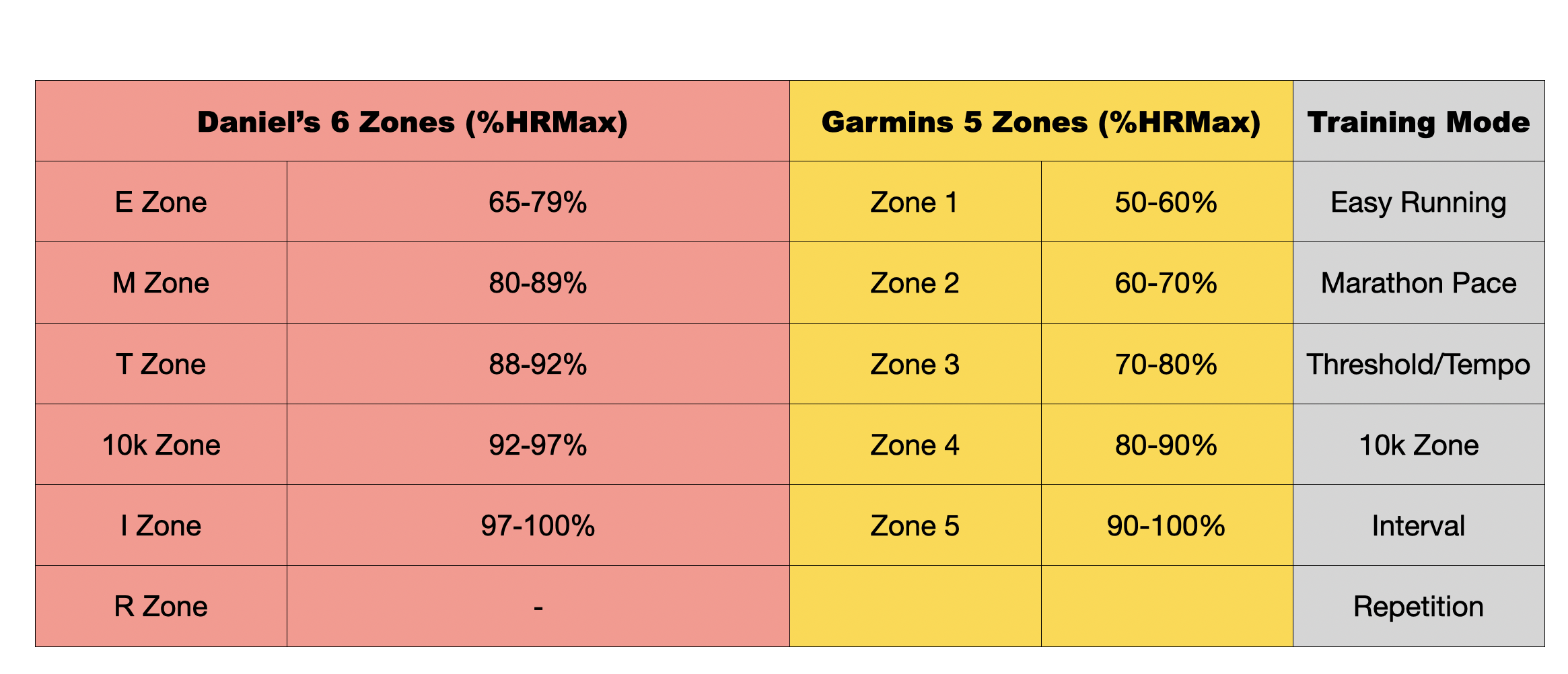
Many runners use the heart rate (HR) data to plan their training strategies. Heart rate is an individual metric and differs between athletes running the same pace, therefore, it can help them to pace themselves properly and can be a useful metric to gauge fatigue and fitness level. One of the most popular systems used by marathon trainers including the heart rate are the ones introduced by Daniels Running Formula and those adopted by Garmin services; in both they define zones taking account the maximum heart rate and resting heart rate. These zones are broad for the convenience of the athlete when performing workouts at a given intensity. This intensity should vary depending on the purpose of the workout (recovery, threshold, VO2 max intervals , etc.).
Below, we present the zones using percentage of maximum heart rate (HRmax) as cuttofs.
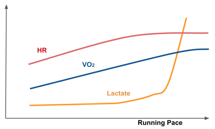
But why heart rate is an important marker of running effort ? Studies suggest that the human running is an energy transfer process. Running economy can be measured by how fast one can run, given a level of oxygen consumption (VO2). VO2 level is almost linearly correlated with running pace (effort) and high correlated with heart rate. The new devices provide HR recordings and it is easier to measure the HR instead of other markers.
For many experienced runners, it would be important to analyze your historical workouts, explore your heart rate range variation and check the ellapsed time through each training zone in order to ensure that you are running at the right effort level to maximize your workout. In this post we will present how we can explore our heart rate (HR) records and the respective training zones based on the data provided from the smartwatches or tracking running apps.
The easiest way resorts to a empirical equation, HRmax = 220 - Age. It is drawn from some epidemiological studies; thus, may not personalized. A better way is to monitor HR while running uphill intervals or use your historical data to compute your HRmax. In this scenario let's use the empirical HRmax. My current age is 36, so my max heart rate would be 184 (HRmax = 220-36).
As we explained above, the heart rate is grouped by zones: active recovery (easy running), general aerobic (marathon pace), basic endurance or the lactate threshold zone (tempo run) and the anaerobic or the VO2 max work(interval). For my maximum heart rate of 184, based on the Garmin's thresholds, the zones can be calculated as:
| Zone | heart_rate | |
|---|---|---|
| Z1 (Active recovery) | 110 | |
| Z2 (Endurance) | 129 | |
| Z3 (Tempo) | 147 | |
| Z4 (Threshold) | 166 | |
| Z5 (VO2 Max) | 184 |
Now that we have the training zones, by using runpandas we could play with our workouts and evaluate the quality of the workouts based on its training zones.
In this example, I selected one of my workouts to further explore these zones and how they correlate with the sensors data available recorded.
import runpandas
activity = runpandas.read_file('./data/11km.tcx')
print('Start', activity.index[0],'End:', activity.index[-1])
print(activity.iloc[0]['lat'], activity.iloc[-1]['lat'])
First, let's perform a QC evaluation on the data, to check if there's any invalid or missing data required for the analysis. As you can see in the cell below, there are 5 records with heart rate data missing. We will replace all these with the first HR sensor data available.
import numpy as np

group_hr = activity['hr'].isnull().sum()
print("There are nan records: %d" % group_hr)

#There is 5 missing values in HR. Let's see the positions where they are placed in the frame.
print(activity[activity['hr'].isnull()])

#We will replace all NaN values with the first HR sensor data available
activity['hr'].fillna(activity.iloc[5]['hr'], inplace=True)

print('Total nan after fill:', activity['hr'].isnull().sum())
The same QC method will be applied on the elevation , speed and distance sensor data. However, to fill the missing data we will apply a special method
in pandas.DataFrame.fillna with the method='ffill' option. 'ffill' stands for 'forward fill' and will propagate last valid observation forward.
group_alt = activity['alt'].isnull().sum()
print("There are nan records: %d" % group_alt)

#There is 16 missing values in HR. Let's see the positions where they are placed in the frame.
print(activity[activity['alt'].isnull()])

#We will replace all NaN values with the last valid alt sensor data available
activity['alt'].fillna(method='ffill', inplace=True)

print('Total nan after fill:', activity['alt'].isnull().sum())
group_dist = activity['dist'].isnull().sum()
print("There are nan records: %d" % group_dist)

#There is non missing values in distance series.
print(activity[activity['dist'].isnull()])


group_speed = activity['speed'].isnull().sum()
print("There are nan records: %d" % group_speed)

#There is non missing values in speed series.
print(activity[activity['speed'].isnull()])
The first question is to see how my heart data changed over time during my workout. In the figure below I present my heart data varying as a function time. For plotting the data I have used the matplotlib package.
import pandas as pd
import numpy as np
import matplotlib.patches as mpatches
from matplotlib import pyplot as plt
plt.style.use('seaborn-poster')


ZONE_COLORS_0 = {
    1: '#ffffcc',
    2: '#a1dab4',
    3: '#41b6c4',
    4: '#2c7fb8',
    5: '#253494'
}

def format_time_delta(time_delta):
    """Create string after formatting time deltas."""
    timel = []
    for i in time_delta:
        hours, res = divmod(i, 3600)
        minutes, seconds = divmod(res, 60)
        timel.append('{:02d}:{:02d}:{:02d}'.format(int(hours), int(minutes),
                                                   int(seconds)))
    return timel

def _make_time_labels(delta_seconds, nlab=5):
    """Make n time formatted labels for data i seconds"""
    label_pos = np.linspace(min(delta_seconds), max(delta_seconds),
                            nlab, dtype=np.int_)
    label_lab = format_time_delta(label_pos)
    return label_pos, label_lab

def heart_rate_zone_limits(maxpulse=187):
    """Return the limits for the heart rate zones."""
    lims = [(0.5, 0.6), (0.6, 0.7), (0.7, 0.8), (0.8, 0.9), (0.9, 1.0)]
    return [(maxpulse * i[0], maxpulse * i[1]) for i in lims]

def plot_hr(data, maxpulse=184):
    """Plot the heart rate per time with training zones."""
    fig = plt.figure()
    ax1 = fig.add_subplot(111)
    ax1.set_facecolor('0.90')
    xdata = data.index.total_seconds().tolist()
    ydata = data['hr'].tolist()
    handles = []
    legends = []
    zones = heart_rate_zone_limits(maxpulse=maxpulse)
    for i, zone in enumerate(zones):
        patch = mpatches.Patch(color=ZONE_COLORS_0[i+1])
        legend = 'Zone = {}'.format(i + 1)
        handles.append(patch)
        legends.append(legend)
        ax1.axhspan(zone[0], zone[1], color=ZONE_COLORS_0[i+1])
    ax1.plot(xdata, ydata, color='#262626', lw=3)
    ax1.legend(handles, legends)
    ax1.set_ylim(min(ydata) - 2, max(ydata) + 2)
    label_pos, label_lab = _make_time_labels(xdata, 5)
    ax1.set_xticks(label_pos)
    ax1.set_xticklabels(label_lab, rotation=25)
    ax1.set_xlabel('Time')
    ax1.set_ylabel('Heart rate / bpm')
    fig.tight_layout()
    return fig

fig = plot_hr(activity, maxpulse=184)

From the chart we can conclude that during periodic intervals, I had a rapid loss of the heart rate , probably due to a stop during the workout. Another important insight is that my training zone kept most of the time between the Z2-Z3 (endurance-tempo run). But how did the altitude interfer in this variation ?
For this question, based on my elevation profile (the altitude variation) as a function time, I plot the elevation against function of time to check the influence of the altitude.
def find_regions(yval):
    """Find borders for regions with equal values.
    Parameters
    ----------
    yval : array_like
        The values we are to locate regions for.
    Returns
    -------
    new_regions : list of lists of numbers
        The regions where yval is constant. These are on the form
        ``[start_index, end_index, constant_y]`` with the
        interpretation that ``yval=constant-y`` for the index
        range ``[start_index, end_index]``
    """
    regions = []
    region_y = None
    i = None
    for i, ypos in enumerate(yval):
        if region_y is None:
            region_y = ypos
        if ypos != region_y:
            regions.append([i, region_y])
            region_y = ypos
    # for adding the last region
    if i is not None:
        regions.append([i, region_y])
    new_regions = []
    for i, region in enumerate(regions):
        if i == 0:
            reg = [0, region[0], region[1]]
        else:
            reg = [regions[i-1][0], region[0], region[1]]
        new_regions.append(reg)
    return new_regions


def calculate_hr_zones(data, max_heart_rate=184):
    limits = heart_rate_zone_limits(max_heart_rate)
    bins = [i[0] for i in limits]
    hr_zone = np.digitize(data['hr'], bins, right=False)
    hr_zone_limis = find_regions(hr_zone)
    return hr_zone_limis


def plot_elevation_hrz(track_name, track_type, data):
    """Plot the elevation profile with heart rate annotations."""
    fig = plt.figure()
    ax1 = fig.add_subplot(111)
    ax1.set_facecolor('0.90')
    ax1.set_title('{}: {}'.format(track_name, track_type))
    xdata = data.index.total_seconds().tolist()
    ydata = data['alt'].tolist()
    ax1.plot(xdata, ydata, color='#262626', lw=3)
    handles = []
    legends = []
    for i in calculate_hr_zones(activity):
        xpos = xdata[i[0]:i[1]+1]
        ypos = ydata[i[0]:i[1]+1]
        ax1.fill_between(xpos, 0, ypos, alpha=1.0,
                         color=ZONE_COLORS_0[i[2]])
    for i in range(1, 6):
        patch = mpatches.Patch(color=ZONE_COLORS_0[i])
        legend = 'Zone = {}'.format(i)
        handles.append(patch)
        legends.append(legend)
    ax1.legend(handles, legends)
    ax1.set_ylim(min(ydata) - 2, max(ydata) + 2)
    label_pos, label_lab = _make_time_labels(xdata, 5)
    ax1.set_xticks(label_pos)
    ax1.set_xticklabels(label_lab, rotation=25)
    ax1.set_xlabel('Time')
    ax1.set_ylabel('Elevation / m')
    fig.tight_layout()
    return fig

fig = plot_elevation_hrz(track_name='Sanharo 11km', track_type='Running', data=activity)

As we can see at the chart, some intervals due to the elevation gain , the effort is increasingly accordingly, which hits my heart rate. Probably, while running into some elevation, the height and speed increasingly difficult my heart to get enough oxygen to my muscles. Now, let's see whether the speed also take effect in my heart rate variation.
In the plot below, it shows the correlation between speed x altitude x heart rate. The velocity keeps steadily along all the workout, but when there is a elevation gain and the speed keeps the same, probably there is a variation on my heart rate (Zone Z3 to Zone Z4).
plt.style.use('seaborn-talk')


def smooth(signal, points):
    """Smooth the given signal using a rectangular window."""
    window = np.ones(points) / points
    return np.convolve(signal, window, mode='same')

def plot_dist_hr_velocity(data):
    fig = plt.figure()
    ax1 = fig.add_subplot(111)

    x = activity['dist'].tolist()
    y = activity['alt'].tolist()

    line1, = ax1.plot(x, y, lw=5)
    # Fill the area:
    ax1.fill_between(x, y, y2=min(y), alpha=0.3)
    ax1.set(xlabel='Distance / km', ylabel='Elevation')
    # Add heart rate:
    ax2 = ax1.twinx()
    # Smooth the heart rate for plotting:
    z = data['hr'].tolist()
    heart = smooth(z, 51)
    line2, = ax2.plot(x, heart, color='#1b9e77', alpha=0.8, lw=5)
    ax2.set_ylim(0, 200)
    ax2.set(ylabel='Heart rate / bpm')
    # Add velocity:
    ax3 = ax1.twinx()
    ax3.spines['right'].set_position(('axes', 1.2))
    # Smooth the velocity for plotting:
    velocity = data['speed']
    vel = 3.6 * smooth(velocity, 51)
    line3, = ax3.plot(x, vel, alpha=0.8, color='#7570b3', lw=5)
    ax3.set(ylabel='Velocity / km/h')
    ax3.set_ylim(0, 20)

    # Style plot:
    axes = (ax1, ax2, ax3)
    lines = (line1, line2, line3)
    for axi, linei in zip(axes, lines):
        axi.yaxis.label.set_color(linei.get_color())
        axi.tick_params(axis='y', colors=linei.get_color())
        key = 'right' if axi != ax1 else 'left'
        axi.spines[key].set_edgecolor(linei.get_color())
        axi.spines[key].set_linewidth(2)

    ax1.spines['top'].set_visible(False)

    for axi in (ax2, ax3):
        for key in axi.spines:
            axi.spines[key].set_visible(False)
        axi.spines['right'].set_visible(True)

    # Add legend:
    ax1.legend(
            (line1, line2, line3),
            ('Elevation', 'Heart rate', 'Velocity'),
            loc='upper left',
            frameon=False
    )

fig = plot_dist_hr_velocity(activity)

Finally, let's see how many minutes were spent in each HR zone. The plot below shows that most time of the training my heart was between Z3 and Z4 zones.
from matplotlib.cm import get_cmap

plt.style.use('seaborn-talk')

def get_limits_text(max_heart_rate=184):
    limits = heart_rate_zone_limits(max_heart_rate)
    txt = {
        0: f'$<${int(limits[0][0])} bpm',
        1: f'{int(limits[0][0])}‒{int(limits[0][1])} bpm',
        2: f'{int(limits[1][0])}‒{int(limits[1][1])} bpm',
        3: f'{int(limits[2][0])}‒{int(limits[2][1])} bpm',
        4: f'{int(limits[3][0])}‒{int(limits[3][1])} bpm',
        5: f'$>${int(limits[3][1])} bpm',
    }
    return txt

def plot_hr_distribution(data):
    fig = plt.figure()
    ax1 = fig.add_subplot(111)

    time = data.index.total_seconds().tolist()
    time_in_zones = {}
    for start, stop, value in calculate_hr_zones(activity):
        seconds = (time[stop] - time[start])
        if value not in time_in_zones:
            time_in_zones[value] = 0
        time_in_zones[value] += seconds
    sum_time = sum([val for _, val in time_in_zones.items()])
    # Check consistency:
    print('Times are equal?', sum_time == (time[-1] - time[0]))

    zone_txt = get_limits_text()

    zones = sorted(list(time_in_zones.keys()))
    percent = {
        key: 100 * val / sum_time for key, val in
        time_in_zones.items()
    }
    labels = [
        f'Zone {i} ({zone_txt[i]})\n({percent[i]:.1f}%)' for i in zones
    ]
    values = [time_in_zones[i] for i in zones]
    times = format_time_delta(values)
    cmap = get_cmap(name='Reds')
    colors = cmap(np.linspace(0, 1, len(zones) + 1))
    colors = colors[1:]  # Skip the first color
    rects = ax1.barh(zones, values, align='center', tick_label=labels)
    for i, recti in enumerate(rects):
        recti.set_facecolor(colors[i])
        width = int(recti.get_width())
        yloc = recti.get_y() + recti.get_height() / 2
        ax1.annotate(
                times[i],
                xy=(width, yloc),
                xytext=(3, 0),
                textcoords="offset points",
                ha='left', va='center',
                fontsize='x-large'
        )
    ax1.spines['top'].set_visible(False)
    ax1.spines['right'].set_visible(False)
    ax1.spines['bottom'].set_visible(False)
    ax1.tick_params(bottom=False)
    ax1.tick_params(labelbottom=False)
    fig.tight_layout()
    return fig

fig = plot_hr_distribution(activity)

With the plots produced at hand, I could check if the training was effective. In this workout, I found out, that I could set my heart rate alert to check when I have to leave the zone by running faster or slower depending on my workout plan and how the altitude had a play in my heart rate variation.
In future releases, we will provide special methods to runpandas in order to compute the training zones to each record in the activity and the time spent in each zone. We are also planning special plots like those above to be called directly from the package. Stay tunned!