Understanding moving time vs ellapsed time, distance and speed/pace calculations
How the tracking apps analyse the GPS activity data


Sport tracking applications and the social networks are quite popular among the runners nowadays. Everyone wants to perform the best run looking for a better pace, distance or time. But have you wondered how these metrics are calculated ?
In this post we’ll use gpx-file downloaded from Strava social application, extract, and analyse the gpx data of one single route. We’ll start with extracting the data from the gpx-file into a convenient runpandas.Activity dataframe. From there we’ll explore the data and try to replicate the stats and graphs that the interface of one most popular running application provides us with.
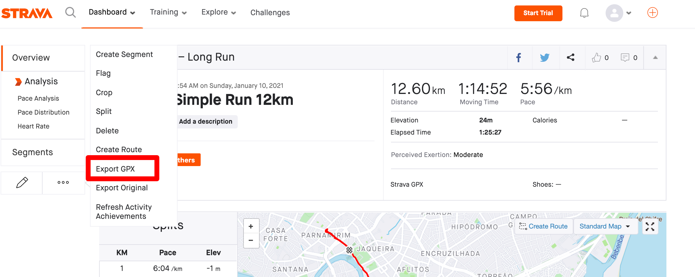
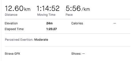
Most of the popular tracking apps allow you to download your activity as a gpx or tcx file. In this post, we will analyse a 12km run from Strava. The gpx-file, short for GPS Exchange Format, can usually be obtained by clicking on export. The screenshot below shows you where you can download your gpx-file in Strava. You can download the file used in this article here.
Now, we want to load our gpx data into a runpandas.Activity. Take a look at your start point and end point and make sure everything makes sense (i.e. start time < end time). If not, there might be something wrong with your data, or you might have forgotten about some tracks or segments.
import runpandas
activity = runpandas.read_file('./data/post-metrics.gpx')
print('Start', activity.index[0],'End:', activity.index[-1])
print(activity.iloc[0]['lat'], activity.iloc[-1]['lat'])
The head of the activity (frame) should look like this:
activity.head(8)
It is important to notice that the time interval between two data points isn't constant. This happens because the device which records the data can't always provide the GPS-data due to connectivity problems or even to hardware limitation. In case of such a failure/limitation the data point is skipped (without an error) and the app will collect the data at the next time interval. So keep in mind that for further analysis we can't assume that the interval between all points is the same.
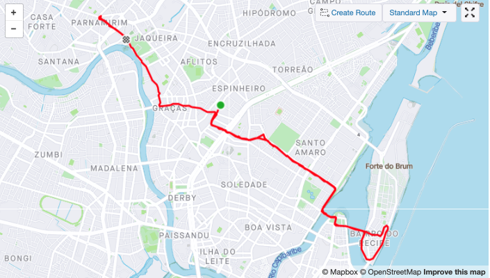
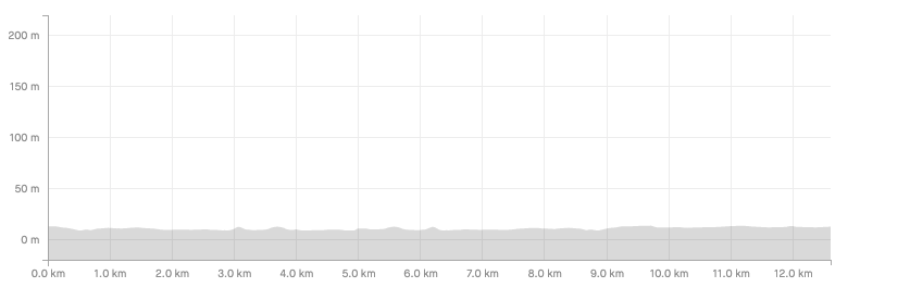
Now with the data loaded, we can explore it with some basic plots. Strava provides some interesting graphs to the runner such as the 2D map (longitude vs latitude) and elevation gain during the activity (altitude vs time). Using native plotting tools we can come to quite similar results.
import matplotlib.pyplot as plt
plt.plot(activity['lon'], activity['lat'])

axis = activity.plot.area(y='alt')
axis.set_ylim(0,100)

Now let's going through the key metrics of the activity such as distance and speed. A quick look can misguide you into incorrect calculations. The first one is the distance between two LL-points (latitude, longitude) which it isn't a straight line, but spherical.
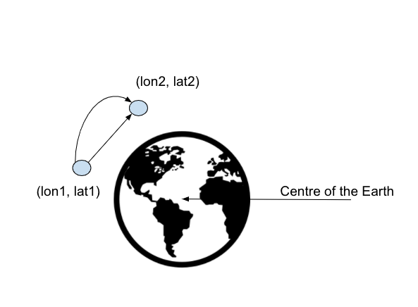
There are two main approaches to calculate the distance between two points on a spherical surface: the Haversine distance and the Vincenty distance. The two formulas take a different approach on calculating the distance, but this is outside the scoop of this post. The maths behind both approaches can be found here.
Another issue about the distance calculation is if the data have been calculated solely based on latitude and longitude, without taking into consideration the elevation gain or loss, then the distance covered can be underestimated. The easiest way to do this, is to compute the spherical 2d distance and then use the Euclidean formula to add the altitude measurements. The formula below shows this last step.
If the uncorrected distance covered at time point $t_{i}$ is $d_{2,i}$, to correct the distance covered between time point $t_{i-1}$ and time point $t_{i}$ to \begin{equation} d_{i} - d_{i-1} = \sqrt{ \left(d_{2,i} - d_{2,i-1} \right)^{\!\!2} + \left(a_{i} - a_{i-1} \right)^{\!\!2}} \end{equation} , where $d_{i}$ and $a_{i}$ are the corrected cumulative distance and the altitude at time $t_{i}$, respectively.
Now with the theoretical background presented, we can start implementing these formulas in our code. We will apply in all data points all possible implementations of our distance formula (Haversine or Vicenty and 2d or 3d) and compute the total distance for every data point by using the dataframe function cumsum.
There are geodesic python libraries already available with Vicenty and Haversine formulas, so we will import them here for our distance calculations.
#pip install haversine & pip install vincenty
from vincenty import vincenty as vn
from haversine import haversine as hv
from haversine import Unit
import numpy as np
activity['shift_lon'] = activity.shift(1)['lon']
activity['shift_lat'] = activity.shift(1)['lat']
#compute the vincenty 2d distance
activity['distance_vin_2d'] = activity[['lat', 'lon', 'shift_lat', 'shift_lon']].apply(lambda x: vn( (x[0], x[1]),(x[2], x[3])), axis=1)
#transform the value in meters
activity['distance_vin_2d'] = activity['distance_vin_2d'] * 1000
#compute the haversine 2d distance
activity['distance_hav_2d'] = activity[['lat', 'lon', 'shift_lat', 'shift_lon']].apply(lambda x: hv((x[0], x[1]),(x[2], x[3]), unit=Unit.METERS), axis=1)
#compute the total distance
activity['distance_vin_no_alt'] = activity['distance_vin_2d'].cumsum()
activity['distance_hav_no_alt'] = activity['distance_hav_2d'].cumsum()
#compute the vincenty and haversine 3d
activity['shift_alt'] = activity.shift(1)['alt']
activity['alt_dif'] = activity[['alt', 'shift_alt']].apply(lambda x: x[1] - x[0], axis=1)
activity['distance_vin_3d'] = activity[['distance_vin_2d', 'alt_dif']].apply(lambda x: np.sqrt(x[0]**2 + (x[1])**2), axis=1)
activity['distance_hav_3d'] = activity[['distance_hav_2d', 'alt_dif']].apply(lambda x: np.sqrt(x[0]**2 + (x[1])**2), axis=1)

#compute the total distances for vincenty and haversined 3D
activity['distance_vin'] = activity['distance_vin_3d'].cumsum()
activity['distance_hav'] = activity['distance_hav_3d'].cumsum()

activity.drop(['shift_lon', 'shift_lat', 'shift_alt'], axis=1)
#present the results
activity[['distance_vin', 'distance_hav', 'distance_hav_3d', 'distance_vin_3d']]
For futher convenice, we can extract the data in our previously created activity. Let's check the results with the following print comand.
print('Vicenty 2D: ', activity['distance_vin_no_alt'].max())
print('Haversine 2D: ', activity['distance_hav_no_alt'].max())
print('Vincenty 3D: ', activity['distance_vin'].max())
print('Haversine 3D: ', activity['distance_hav'].max())
If we compare the distance calculations between the app and ours, we will see they are almost similar.
But why do we have 50m of difference between our internal calculations and the distance showed in the app ? It is explained in an article from Strava's support team.
In this scenario our 2d calculations are right and the we might conclude the app doesn’t take elevation into account. The difference between the distance proposed by the app and our estimate is about 50m (0.03%). Note that this difference will increase if you undertake more altitude-intense activities (mountain biking or hiking).
Now let's going forward to our next metric, the total activity time ellapsed x moving time.
def strfdelta(tdelta, fmt):
    d = {"days": tdelta.days}
    d["hours"], rem = divmod(tdelta.seconds, 3600)
    d["minutes"], d["seconds"] = divmod(rem, 60)
    return fmt.format(**d)

print('Total time: ' , strfdelta(activity.index[-1], "{hours} hour {minutes} min {seconds} sec"))
The total time elapsed totally agrees with our calculations, but the moving time seems to be diferent. Let us explain the basic concepts: Elapsed time is the duration from the moment you hit start on your device or phone to the moment you finish the activity. It includes stoplights, coffee breaks, bathroom stops and stopping for photos. Moving time, on the other hand, is a measure of how long you were active, this can be realistic when we have to slow down and stop for a traffic light, for example.
Let’s see if we can figure out which threshold Strava uses to stop the timer (and therefore boost our average speed). To do so, we need to create a new variable that calculates our movement in meters per second (and not just movement per data point, hence why we created the time difference variable). Let’s do this for our haversine 2d distance, since that’s the closest approximation of the distance proposed by the app.
import pandas as pd
import numpy as np
activity['time'] = activity.index
activity['time_dif'] = (activity.time - activity.time.shift(1).fillna(activity.time.iloc[0]))/np.timedelta64(1,'s')
activity['distance_dif_per_sec'] = activity['distance_hav_2d'] / activity['time_dif']
activity['distance_dif_per_sec']
With this new variable we can iterate through a list of thresholds. Let's assume values between 50 cm and 1 meter, and try to evaluate which one adds up to a timer time-out closest to 640 seconds (~=10 minutes).
for treshold in [0.5, 0.6, 0.7, 0.8, 0.9, 1]:
    print(treshold, 'm', ' : Time:',
          sum(activity[activity['distance_dif_per_sec'] < treshold]['time_dif']),
         ' seconds')
As we can see at the table above, the movement per second was less than 80-70 centimeters, the application didn't consider it as movement and discard those intervals (it's about 2.9 km/h , a speed far below that most people do in their walking pace). Since we don't have the algorithm used for the real calculation in the app, we can get to an approximate moving time.
total_time = activity['time_dif'].sum()
stopped_time =  sum(activity[activity['distance_dif_per_sec'] < 0.8]['time_dif'])
pd.Timedelta(seconds=total_time - stopped_time)
With the moving time and distance calculated, we can now calculate the pace and speed. Speed is calculated by dividing the distance traveled in meters by the time it took in seconds, and then converted to km/h.
activity['speed'] = (activity['distance_hav_2d'] / activity
['time_dif']) * 3.6
Next we will filter out all the data where the movement per second is larger than 80 centimeters, based on the threshold we evaluated above.
activity_with_timeout = activity[activity['distance_dif_per_sec'] > 0.8]
Finally, we compute the weighted average speed and convert it to minutes and seconds per kilometers to get the Pace metric.
def pace(speed, fmt):
    d = {"hours": 0}
    d["minutes"] = np.floor(60 / speed)
    d["seconds"] = round(((60 / speed - np.floor(60 / speed))*60), 0)
    return fmt.format(**d)

avg_km_h = (sum((activity_with_timeout['speed'] *
                 activity_with_timeout['time_dif'])) /
            sum(activity_with_timeout['time_dif']))

print('Speed:', avg_km_h , 'km/h')
print('Cadence:' , pace(avg_km_h, "{hours} hour {minutes} min {seconds} sec"))
The results compared to the proposed by our app show similar values, with average speed of 5 minutes and 58 seconds per kilometer, a difference of only just 2 secs.
Let's plot our average speed for every 10 seconds to see our speed floats during the run. For this plot we will need the cumulative sum of our time differente to 10 seconds and plot the aggregated speed against it.
activity['time_10s'] = list(map(lambda x: round(x, -1), np.cumsum(activity['time_dif'])))
plt.plot(activity.groupby(['time_10s']).mean()['speed'])

The result shown is a smooth line plot where we check the speed (km/h) vs the time in seconds.
The last metric we will explore is the elevation gain. According to the apps documentation, the cumulative elevation gain refers to the sum of every gain elevation throughout an entire Activity.
Based on that, we can compute the elevation gain by mapping over our altitude difference column of our dataframe.
activity_with_timeout.loc[activity_with_timeout['alt_dif'] > 0]['alt_dif'].sum()
The elevation calculated is far away from what the app showed (about 25m). Checking the altitude difference column values we can see that there are measures down to 10 centimeters. After reading the docummentation, we found out that the elevation data go through a noise correction algorithm. It is based on the a threshold where climbing needs to occur consistently for more than 10 meters for activities without strong barometric or two meters for an activity with the barometric data before it's added to the total elevation gain.
elevations = zip(list(activity_with_timeout['alt']), list(activity_with_timeout['distance_hav_2d']))

THRESHOLD_METERS = 10
def calculate_elevation_gain(elevations):
    elevations = list(elevations)
    thresholdStartingPoint = elevations[0][0]
    diff_distance = 0
    count_diff = 0
    gain = 0
    valueAgainstThreshold = 0
    for elevation, distance in elevations:
        diff = elevation - thresholdStartingPoint
        diff_distance+=distance
        if diff > 0:
            valueAgainstThreshold += diff
            if abs(diff_distance) >= THRESHOLD_METERS:
                gain += valueAgainstThreshold
                diff_distance = 0
                valueAgainstThreshold = 0
        else:
            diff_distance = 0
            valueAgainstThreshold = 0
        thresholdStartingPoint = elevation

    return gain

#plt.plot(activity['alt_dif'])
print(calculate_elevation_gain(elevations))
The new result is 25.2m, very close to the elevation propose by the app. Based on that, we could recalculate the 3rd distances to get these new elevation values into account to get the distance closest to the 2d distance.
In this article we presented some popular metrics in runner's world such as moving time, cadence, pace and elevation gain. The calculations behind the metrics were also detailed and we gave a possible approximation of some of the algorithms used by a famous tracking running application, since we don't have access, of course,how they implemented it.
The next steps will be implement these metrics as properties, methods of the runpandas.Activity dataframe. We will release it soon with examples detailed at one of our future posts. Keep following here!
— Please feel free to bring any inconsistencies or mistakes by leaving a comment below.-